Announcements and Demos
-
If you’re struggling with the C syntax, don’t worry, it’s normal! In a few weeks, you’ll look back on Problem Set 2 and be amazed at how far you’ve come.
Searching
-
Imagine there are 7 doors with numbers behind them and you want to find the number 50. If you know nothing about the numbers, you might just have to open the doors one at a time until you find 50 or until all the doors are opened. That means it would take 7 steps, or more generally, n steps, where n is the number of doors. We might call this a linear algorithm.
-
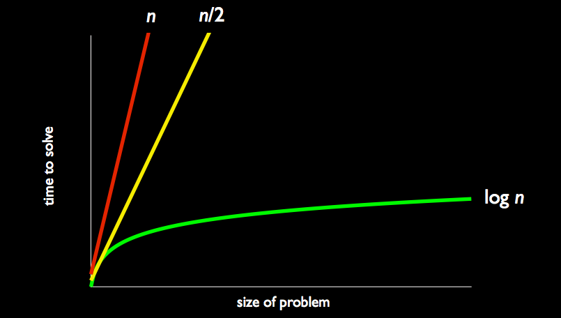
How might our approach change if we know that the numbers are sorted? Think back to the phonebook problem. We can continually divide the problem in half! First we open the middle door. Let’s say it’s 16. Then we know that 50 should be in the doors to the right of the middle, so we can throw away the left. We then look at the middle door in the right half and so on until we find 50! This algorithm has logarithmic running time, the green line in the graph below:
-
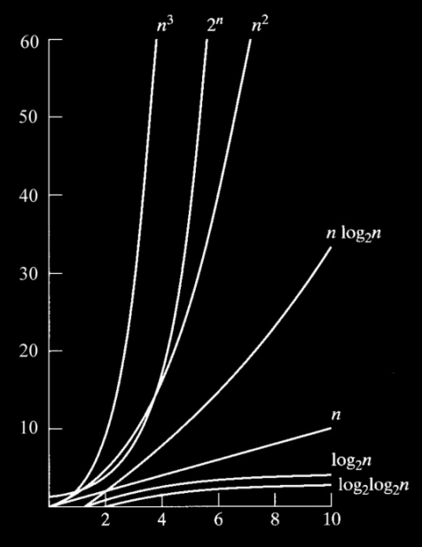
Note that there are plenty of algorithms that are much worse than linear, as this graph shows:
-
Although it looks like n3 is the worst, 2n is much worse for large inputs.
Sorting
Bubble Sort
-
If the numbers aren’t sorted to begin with, how much time will it take to sort them before we search?
-
To start figuring this out, let’s bring 7 volunteers on stage and have them hold pieces of paper with the numbers 1 through 7 on them. If we ask them to sort themselves, it seems to only take 1 step as they apply an algorithm something like "if there’s a smaller number to my right, move to the right of it." In reality, though, it takes more than 1 step as there are multiple moves going on.
-
In order to count the number of steps this algorithm takes, we’ll slow it down and allow only 1 move to happen at a time. So walking left to right among the volunteers, we examine the two numbers next to each other and if they’re out of order, we swap them. We may have to walk left to right more than 1 time in order to finish sorting. How do we know when they’re sorted? As a human, you can look at it and know, but we need a way for the computer to know. If we walk left to right among the volunteers and make 0 swaps, then we can be sure that all the numbers are in the right order. That means we’ll need to store the number of swaps made in a variable that we check after each walkthrough.
-
This algorithm we just described is called bubble sort. To describe its running time, let’s generalize and say that the number of volunteers is n. Each time we walk through the volunteers, we’re taking n-1 steps. Let’s just round that up and call it n. How many times do we walk left to right through the volunteers? In the worst case scenario, the numbers will be perfectly out of order, that is, arranged left to right largest to smallest. In order to move the 1 from the right side all the way to the left side, we’re going to have to walk through the volunteers n times. So that’s n steps per walkthrough and n walkthroughs, so the running time is n2.
Selection Sort
-
Another approach we might take is to walk through the volunteers left to right and keep track of the smallest number we find. After each walkthrough, we then swap that smallest number with the leftmost number that hasn’t been put in its correct place yet. On each walkthrough, we start one position to the right of where we started on the walkthrough before so as not to swap out a number we already put in its correct position.
-
This algorithm is called selection sort. Here’s what our numbers look like after each walkthrough:
4 2 6 1 3 7 5 1 2 6 4 3 7 5 1 2 6 4 3 7 5 1 2 3 4 6 7 5 1 2 3 4 6 7 5 1 2 3 4 5 7 6 1 2 3 4 5 6 7 -
So which algorithm is faster, bubble sort or selection sort? With selection sort, we’re again going to have to do n walkthroughs in the worst case. On the first walkthrough, we take n-1 steps. On the second walkthrough, because we know that the leftmost number is in its correct position, we start at the second lefmost and we take n-2 steps. On the third walkthrough, we take n-3 steps. And so on. So our total running time is n-1 + n-2 + n-3 + n-4… which works out to be (n(n-1)) / 2. Although this is less than n2, as n gets very large, the difference between the two is negligible. So we say that selection sort’s running time is also n2 and thus it has the same running time as bubble sort.
Insertion Sort
-
Our next approach will be to sort the numbers in place. When examining each element, we place it in its correct position in a smaller list on the left that we’ll call the sorted list. Observe:
4 2 6 1 3 7 5 4 2 6 1 3 7 5 2 4 6 1 3 7 5 2 4 6 1 3 7 5 1 2 4 6 3 7 5 1 2 3 4 6 7 5 1 2 3 4 5 6 7 1 2 3 4 5 6 7 -
Note that the space is merely to delimit the sorted list from the rest of the list, but the total list is still only size 7.
-
This algorithm might appear to be faster because we only walk through the list once. However, consider what happens when we have to insert 1 at the beginning of the sorted list. We have to move 2, 4, and 6 to the right to make room. In the worst case, we’ll have to shift the entire sorted list every time we need to insert a number. When you consider this, you can deduce that the running time of this algorithm, insertion sort, is also n2.
-
To see these algorithms in action, check out this visualization. You may need to use Firefox and zoom in to see the control buttons.
Big O Notation
-
Let’s summarize the running times of the algorithms we’ve discussed so far using a table. In so-called big O notation, O represents the worst-case running time and `\Omega` represents the best-case running time.
`\Omega`
O
linear search
1
n
binary search
1
log n
bubble sort
n
n2
selection sort
n2
n2
insertion sort
n2
-
In the best case for linear and binary search, the number you’re looking for is the first one you examine, so the running time is just 1. In the best case for our sorting algorithms, the list is already sorted, but in order to verify that in bubble sort, we need to walk through the list at least once. Unfortunately, to verify that in selection sort, we still have to do n2 walkthroughs, each of which confirms that the smallest number is in the correct position.
-
What about the best case for insertion sort? We’ll fill in that blank next time.
-
Are we doomed to n2 running time for sorting? Definitely not. Check out this visualization to see how fast merge sort is compared to bubble sort, selection sort, and insertion sort. Merge sort leverages the same "divide and conquer" technique that binary search does.